
Every serious business decision eventually runs into three curves. Cost. Revenue. Profit. Strip away the buzzwords, dashboards, and motivational slogans, and real money lives or dies inside how those curves behave as volume and price change.
Mathematical analysis earns its place because none of those curves move in clean, straight lines forever. Fixed costs create pressure early. Volume helps for a while, then capacity cracks show up. Pricing changes can send profit soaring, but only when demand holds.
The point here is not math for math’s sake. The point is building a model sturdy enough to answer questions leadership actually asks:
Get those answers right, and strategy becomes grounded. Get them wrong, and growth becomes a very expensive illusion.
The Three Core Curves That Run A Business
View this post on Instagram
Every operating model, whether written down or not, rests on three functions. Each describes a different part of the same story.
Cost Curve
The cost curve shows total cost as a function of output. A clean starting point splits cost into two buckets.
- Fixed costs (F): rent, base payroll, insurance, core software subscriptions.
- Variable costs (v): materials, packaging, transaction fees, hourly labor tied directly to each unit.
The simplest model looks like:
C(q) = F + vq
The structure of functions like this, along with how they change as variables scale, mirrors the type of applied analysis covered step by step on Qui Si Risolve.
Where:
- C(q) is total cost.
- q is units produced or sold in a period.
- F is fixed cost.
- v is variable cost per unit.
That linear form works surprisingly well early on. It lets teams size break-even, estimate cash burn, and plan initial capacity.
Reality bends the curve as volume grows.
- Overtime, rush shipping, scrap, and rework raise cost per unit at high volume.
- Bulk purchasing, process learning, and automation lower cost per unit at moderate volume.
A more realistic cost model often adds curvature:
C(q) = F + vq + aq²
Here, the sign of a tells a story.
- If a > 0, marginal cost rises with volume. Capacity strain shows up.
- If a < 0, marginal cost falls with volume. Scale efficiencies dominate, at least for a while.
Most businesses experience both phases at different ranges of output. Cost curves flatten, then steepen again.
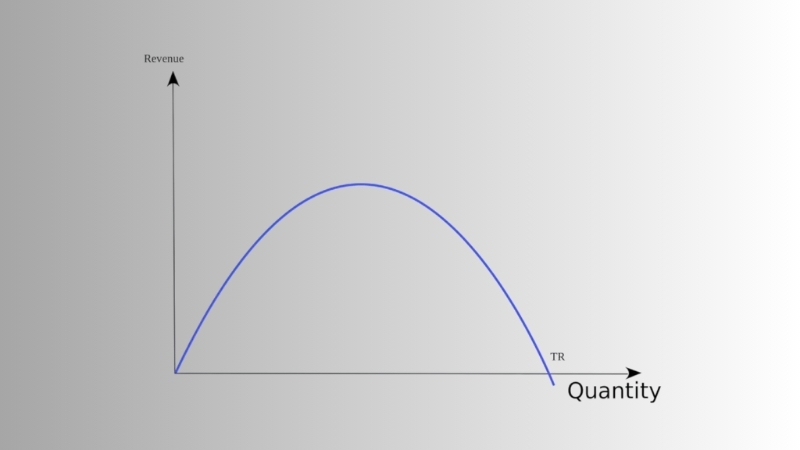
Revenue Curve
Revenue tracks how much money comes in as quantity changes.
If price per unit stays fixed at p, revenue looks simple:
R(q) = pq
Plenty of early-stage forecasts stop here. That works until growth pushes beyond the most eager customers.
As scale increases, price pressure creeps in.
- Discounts to move volume.
- Lower willingness to pay outside the core audience.
- Competitive responses.
A common demand-based model lets price depend on quantity:
p(q) = a − bq
Revenue then becomes:
R(q) = (a − bq)q = aq − bq²
That quadratic shape matters. Revenue rises, peaks, and then falls if volume expansion requires too much price sacrifice.
Profit Curve
Profit pulls the whole picture together.
P(q) = R(q) − C(q)
Strategy lives here. Cost and revenue matter only because of what remains after they collide.
Break-Even Analysis

Break-even happens when sales cover all costs with zero profit or loss
The break-even point marks the output level where profit equals zero. Revenue matches cost.
R = C
It answers the bluntest business question possible. How much needs to sell before the business stops losing money.
The U.S. Small Business Administration formalizes break-even using contribution margin, a standard approach in managerial accounting.
Key Terms That Make Break-Even Work
- Contribution margin per unit (CMu) = price − variable cost.
- Contribution margin ratio (CMR) = contribution margin ÷ price.
The SBA expresses break-even units as fixed costs divided by contribution margin per unit.
Break-Even In Units
Break-even units = F ÷ (p − v)
Break-Even In Sales Dollars
Break-even sales ($) = F ÷ CMR
Where:
CMR = (p − v) ÷ p
A Break-Even Example You Can Drop Into A Forecast
Consider a simple product business.
- Fixed costs per month: $18,000
- Price per unit: $60
- Variable cost per unit: $24
Contribution margin per unit:
CMu = 60 − 24 = $36
Break-even units:
18,000 ÷ 36 = 500 units
Break-even revenue:
500 × $60 = $30,000
Sales at 350 units stay below break-even. Sales at 650 units clear it.
The strategic takeaway is direct. Growth only turns into real profit after fixed costs are covered. Before that point, volume just reduces losses.
Cost-Volume-Profit Analysis
Break-even shows a single point. Cost-volume-profit analysis shows the whole landscape.
CVP links:
- Activity levels.
- Costs.
- Revenue.
- Profit.
Investopedia describes CVP as built around contribution margin and break-even, with the contribution margin ratio used to compute break-even sales dollars.
A Practical CVP Workflow
Step 1: Build The Inputs
- Fixed costs.
- Variable cost per unit.
- Price per unit.
- Expected unit sales range.
- Constraints like capacity, staffing, or supply.
Step 2: Calculate Contribution Margin
Managerial accounting treats the contribution margin in three ways.
- Per unit.
- Total at a given volume.
- As a ratio, showing how much of each sales dollar covers fixed costs.
Step 3: Run What-If Scenarios
Ask questions that leadership actually cares about.
- What happens if price drops 5%?
- What happens if variable cost rises $2?
- What happens if fixed costs jump due to expansion?
CVP turns vague debates into numeric tradeoffs.
Marginal Analysis – The Math Behind “Should We Produce More?”

Profit reaches its highest point at the output level where marginal revenue equals marginal cost
Break-even helps a business survive. Marginal analysis helps it optimize.
In calculus terms:
- Marginal cost (MC) equals the derivative of cost.
- Marginal revenue (MR) equals the derivative of revenue.
- Marginal profit (MP) equals the derivative of profit.
OpenStax explains the business meaning directly. Marginal values come from derivatives of cost, revenue, and profit functions.
The Core Decision Rule
Profit behaves according to three conditions.
- Profit increases when MR > MC.
- Profit peaks when MR = MC, within feasible limits.
- Profit falls when MR < MC.
Translated into operations.
- Each extra unit that costs more than it earns should not be produced.
- Each extra unit that earns more than it costs represents missed profit.
Profit Maximization With A Real Example
Assume the following functions.
Revenue:
R(q) = 120q − 0.4q²
Cost:
C(q) = 10,000 + 30q + 0.1q²
Profit becomes:
P(q) = (120q − 0.4q²) − (10,000 + 30q + 0.1q²)
P(q) = 90q − 0.5q² − 10,000
Take derivatives.
- MR = dR/dq = 120 − 0.8q
- MC = dC/dq = 30 + 0.2q
Set MR equal to MC.
120 − 0.8q = 30 + 0.2q
90 = q
Profit peaks at 90 units.
Interpretation stays practical. At 90 units, the next unit adds the same amount to revenue as it adds to cost. Beyond that, cost rises faster than revenue. Revenue may keep climbing, but profit drops.
Revenue Curves And Pricing Strategy
Revenue rises with price cuts only when demand is elastic enough to offset the lower margin
Total revenue does not always rise when prices fall.
If demand responds strongly to price, lower prices can raise revenue by boosting quantity. If demand barely moves, price cuts shrink revenue.
Economic teaching materials formalize the link between elasticity and marginal revenue. Marginal revenue stays positive when demand remains elastic and turns negative when demand becomes inelastic.
A Practical Pricing Rule
- Elastic demand supports volume-driven revenue gains.
- Inelastic demand supports price-driven revenue gains.
That logic explains why many 10% off promotions disappoint. Volume fails to rise enough to compensate for the lost margin.
Why Small Price Changes Create Huge Profit Swings
Pricing hits profit harder than most teams expect because fixed costs amplify every extra dollar of margin.
McKinsey reports that, on average, a 1% price increase can translate into about an 8.7% increase in operating profits, assuming volume holds.
McKinsey also estimates that up to 30% of pricing decisions fail to deliver the best price, pointing to systematic profit leakage from weak pricing discipline.
Plain meaning for operators.
Once fixed costs are covered, most incremental margin drops straight into operating profit. Pricing work often delivers higher leverage than cost-cutting.
Using Curves To Plan Capacity, Staffing, And Expansion

When capacity strain pushes marginal costs up faster than revenue, profit peaks sooner than planned
Cost curves rarely stay smooth when capacity limits hit.
- New shifts get added.
- Supervisors appear.
- Warehouse space expands.
- Rush fees creep in.
- Quality slips and returns rise.
Mathematically, marginal cost steepens.
Spotting Growth That Hurts
Warning signs show up in the data.
- Variable cost per unit rises at higher volume.
- Fulfillment costs accelerate.
- Support costs spike per sale.
- Churn rises as experience degrades.
If revenue per unit stays flat while marginal cost climbs, profit peaks earlier than expected.
Multi-Product Break-Even: Weighted Contribution Margin
Most businesses sell more than one product.
- Different prices.
- Different variable costs.
- Different margins.
- Different sales mix.
Multi-product CVP handles this by using a weighted average contribution margin ratio. Managerial accounting defines it as total contribution margin divided by total sales.
A Simple Approach
- Calculate contribution margin for each product line.
- Estimate the expected sales mix by revenue or units.
- Compute the blended contribution margin ratio.
Break-even sales dollars become:
Fixed costs ÷ blended CMR
Strategic implication matters. A shift toward lower-margin products raises break-even, even when total revenue looks healthy.
Strategy Depends On Industry Reality

Business strategy must fit industry margins, since low margins need cost control and high margins rely on pricing power
Margin expectations change by sector.
NYU Stern’s Damodaran datasets show wide variation in operating and net margins across industries.
What that means in practice.
- Thin-margin businesses demand tight control over variable costs.
- Pricing errors sting harder.
- Break-even volume often runs high.
High-margin businesses play a different game.
- Willingness-to-pay research matters more.
- Customer acquisition efficiency drives results.
- Retention often beats chasing raw volume.
Benchmarks anchor models in reality rather than wishful thinking.
A Strategy Playbook Built From Curves
Curve analysis pays off when it drives decisions. Here are the highest-value moves it supports.
Choose The Right Profit Lever
Models expose the biggest driver.
- Raise price slightly.
- Reduce variable cost per unit.
- Cut fixed costs.
- Shift product mix.
- Remove low-margin SKUs.
Pricing often stands out once fixed costs are covered, backed by McKinsey’s findings on price and profit.
Stop Chasing Revenue When Marginal Profit Turns Negative
@getparakeeto Midweek reminder: if you’re chasing profit or growth, you’re missing the point. The smartest agencies know how to do both. But how? It starts with understanding the real lever: delivery margin. In this clip, Marcel and Jon Morris break down: ✅ Why the “Rule of 40” still applies (yes, even in services) ✅ Why high EBITDA doesn’t always mean you’re healthy ✅ How to stop starving your growth machine just to “look” profitable ✅ And the metric that actually moves the needle (spoiler: it’s not your net profit) If you’re trying to scale without tradeoffs — this is your blueprint. Go watch it. Then watch the full episode. You won’t look at your financials the same way again. #AgencyGrowth #DeliveryMargin #ProfitVsGrowth #RuleOf40 #EBITDA #AgencyProfitability #AgencyFinance #AgencyOps #AgencyLife #podcasts ♬ original sound – Parakeeto
High revenue with weak contribution margin traps many teams.
Watch for products with:
- Low contribution margin.
- High support costs.
- Elevated returns or churn.
Revenue can grow while results worsen. The math gives a clean test. Negative marginal profit signals damage unless something changes.
Use Break-Even To Time Growth
Break-even defines safety.
- Before break-even, each unit reduces loss.
- After break-even, contribution margin largely converts to profit until constraints appear.
The SBA’s break-even framework helps quantify that threshold using price, variable costs, and fixed costs.
Model Discounts Before Launching Them
Discounts feel easy and reverse poorly.
Run a quick test.
- Old price p₁, old quantity q₁.
- New price p₂, new quantity q₂.
Revenue change:
p₂q₂ − p₁q₁
Profit change:
(p₂ − v)q₂ − (p₁ − v)q₁
Shrinking margin demands a dramatic volume response to pay off.
Use A Decision Table In Leadership Meetings
| Decision | Math Check | What Gets Tested |
| Add Capacity | Does marginal cost rise after a threshold? | Growth constraint cost |
| Run A Discount | Does profit drop even if revenue rises? | Margin vs volume |
| Drop A SKU | Is contribution margin worth the complexity? | Focus efficiency |
| Raise Price | Does volume fall less than margin improves? | Elasticity risk |
| Add Fixed Costs | Does break-even become unrealistic? | Operating leverage |
Common Modeling Mistakes That Break Strategy

Strategy fails when models ignore scaling costs, demand limits, profit focus, and product mix
Even well-intentioned forecasts can quietly sabotage decision-making when small modeling shortcuts distort how cost, revenue, and profit actually behave at scale.
Treating Cost As Only COGS
Support, returns, and service often scale with volume. Ignoring them turns profit curves into fantasy.
Assuming Unlimited Demand At A Fixed Price
Most markets saturate. Revenue curves often peak rather than climb forever.
Optimizing Revenue Instead Of Profit
Revenue can rise while profit falls when marginal cost outpaces marginal revenue.
Ignoring Product Mix
Multi-product break-even requires weighted averages, not a single margin.
A Practical Workflow For Building Curves Without Overengineering

Build curve models step by step and tie each output to real business decisions, not complexity
A practical workflow keeps curve analysis focused on decisions that matter, without burying teams in unnecessary detail or fragile assumptions.
Step 1: Start With A Monthly Model
- Fixed costs (F).
- Variable cost per unit (v).
- Price per unit (p).
- Expected unit range (q).
Step 2: Compute Contribution Margin And Break-Even
Use SBA formulas as the baseline.
Step 3: Add Reality Gradually
Layer in one factor at a time.
- Volume discounts that reduce variable cost.
- Capacity strain that raises variable cost.
- Declining willingness to pay as volume expands.
Step 4: Run Scenario Bands
- Conservative.
- Expected.
- Aggressive.
Step 5: Tie Each Output To A Decision
The model should answer questions like:
- Which price range meets target profit?
- How much volume supports a new hire?
- What discount stays safe?
- Which product line drags blended margin down?
Closing Thoughts

Clear profit, cost, and revenue curves turn strategy into disciplined, data-based decisions instead of guesswork
Profit, cost, and revenue curves turn strategy into something measurable. Disciplined business practices that save time and prevent costly mistakes give those curves practical power in day-to-day execution.
They replace gut feel with structure, without stripping away judgment. A solid model does not promise certainty. It sharpens decisions.
Get the curves roughly right, and strategy becomes disciplined. Ignore them, and growth turns into guesswork with a price tag attached.


